PyTorch is a deep learning framework that significantly simplifies the process of writing and training deep neural networks. It supports a wide range of architectures, from shallow ones to deep ones like transformers. I mean, any neural network architecture you can think of. On the other hand, tensors are fundamental data structures in PyTorch; they are multi-dimensional arrays that serve as the building blocks for designing neural networks. Understanding tensors and the operations you can perform with them is one of the first things you need to learn before delving into building neural networks.
Remember: Neural networks can be trained on literally any kind of data until and unless it can be represented with numbers. Such numbers are generally packed in some ways to form blocks called tensors.
Earlier, I wrote a brief article discussing various ways to represent numerical data: scalars, vectors, matrices, and tensors. If you’ve read the article, it will be particularly beneficial moving forward, as in PyTorch, every data structure is considered a tensor.
Long story short, a scalar is 0th order tensor, a vector is 1st order tensor, and a matrix is 2nd order tensor.
Now, let us see how tensors are created in PyTorch. First, import PyTorch as import torch. Make sure PyTorch is installed in your system before moving forward. There are plenty of resources on the web to help you install PyTorch based on the type of OS you’re using.
Scalars
Here’s a quick example of creating a tensor with a scalar “5”. ndim for the scalar variable returns “0” because scalars are 0th order tensors.

Vectors
Suppose we have the vector [5,9]; we create a tensor as below. ndim gives dimension as “1”, as vectors are 1st order tensors.
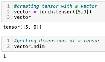
Similarly, for the vector [5,9,2,3]:

Matrices
Now, let us look into matrices, which are 2nd order tensors. Similar to above, we use torch.tensor to create tensors. ndim in this case results “2”. [variable].shape gives the size of the tensor. For the matrix \begin{bmatrix} 1 & 2 & 3\\ 4 & 5 & 6 \end{bmatrix}, we get the shape of the tensor as [2,3] which is fundamentally a 2×3 matrix.

Tensors
Now, let us go further up the dimension. What if there are two 3×3 matrices; something like this: \begin{bmatrix}
\begin{bmatrix}
1 & 2 & 3 \\
4 & 5 & 6 \\
7 & 8 & 9 \\
\end{bmatrix}
,
\begin{bmatrix}
1 & 2 & 3 \\
4 & 5 & 6 \\
7 & 8 & 9 \\
\end{bmatrix}
\end{bmatrix}. Here, if we check the dimensions, ndim returns “3”. Also, if we check the shape of the tensor, we get [2,3,3]; which is basically two 3×3 matrices wrapped together.
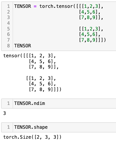
Going further on, we can introduce more dimensions in a similar manner. I hope these examples clarify what tensors are and how they are created using PyTorch. These are just for illustration purposes. In the real world, there are functions in PyTorch that help us create tensors of different shapes. However, it is absolutely necessary to learn what the dimensions mean when dealing with tensors.
Into the wild…
As mentioned earlier, there is no need to manually create tensors. Neural networks begin with randomly initialized tensors (i.e., weights) containing random numbers. As the network progresses based on a certain loss function (let’s say, MSE), the random numbers are adjusted so that after a certain number of iterations, we reach the minimum of the loss function. Please refer to these two articles to delve deeper into how neural networks work and how gradient descent works.
Generating random tensors
We use torch.rand to generate tensors of any size. Some examples are provided below. The random numbers are pulled from a uniform distribution on the interval [0,1).

Similarly, we can generate random tensors for some other sizes. Let us add one more dimension to what we have above.

You can also provide the size this way torch.rand((1,2,3)) or even torch.rand(size=(1,2,3)).
Tensors with Zeros and Ones
The tensors created above with rand were randoms between [0,1). We can also create tensors of different sizes with just zeros or ones as the elements. For tensors with just zeros we use torch.zeros and for the ones we use torch.ones.
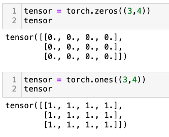
We also have torch.zeros_like and torch.ones_like to copy the structure of an existing tensor and create a new one with just zeros or ones as elements.

Tensors with a range
Suppose you want to create a 1-D tensor with elements starting and ending at specific numbers. Well, torch.arange is what you’ll need.

Tensor Data types
The default data type in PyTorch is float32. Other types, such as float64, float16, int8, int16, int32, int64, bool, etc., are also available. Refer to this page for more details on data types.

As shown above, we can easily change the data type of tensors, and different data types can be operated together.
Type, shape and device: Use [tensor].dtype for checking data type, [tensor].shape for checking the shape, and [tensor].device to check if the tensor is on CPU or GPU.
Tensor Operations with PyTorch
At a theoretical level, I have already covered basic tensor operations in this post: Basic Operations on Tensors. Here, let us see how we can manipulate tensors in code with PyTorch.
Addition/subtraction of tensors:
The examples below are self-explanatory.

Multiplication (element-wise) and division of tensors:
Let us consider the same tensors tensor1 and tensor2 and perform multiplication and division. Here are the results:

If we bring in a scalar and perform multiplication and division, the following are the results:

Matrix multiplication:
For matrix multiplication, the number of columns of the first matrix must match the number of rows of the second matrix.
Here’s an example:
Let’s suppose two matrices, \begin{pmatrix} 1 & 2 & 3\\ 4 & 5 & 6 \end{pmatrix} and \begin{pmatrix} 1 & 2 \\ 3 & 1\\ 2 & 3 \end{pmatrix}
= \begin{pmatrix} 1 & 2 & 3\\ 4 & 5 & 6 \end{pmatrix} * \begin{pmatrix} 1 & 2 \\ 3 & 1\\ 2 & 3 \end{pmatrix} \\ = \begin{pmatrix} 1*1+2*3+3*2 & 1*2+2*1+3*3\\ 4*1+5*3+6*2 & 4*2+5*1+6*3 \end{pmatrix} = \begin{pmatrix} 13 & 13\\ 31 & 31 \end{pmatrix}Multiplication of a matrix and a vector (column vector) is also possible until the dimension conditions match.
In PyTorch, we can use torch.matmul to perform matrix multiplication as below:

Transpose tensors:
Sometimes we might need to transpose tensors; for instance, turn a 2×3 matrix into a 3×2. In that case, you can use [tensor].T where T means transpose.
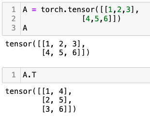
Tensor aggregation:
So you have a tensor and would want to find out the minimum, maximum, mean and sum of the elements in the tensor; we have multiple methods in PyTorch for these tasks. Here are some examples:

We also have [tensor].argmin and [tensor].argmax to find the position of the minimum and the maximum in a tensor. Here’s an example:

The lowest value in the tensor is 0.1769 at 4th position, and the maximum value in the tensor is 0.9471 at 13th position.
Restructuring of tensors:
The restructuring of tensors includes tasks such as reshaping, viewing, stacking (verticle and horizontal), squeezing, unsqueezing, and permuting. Let us see how these tasks affect tensors.
Reshaping: A tensor is reshaped to a different compatible shape. For instance, in the example below, with a tensor of size 10, PyTorch gives an error if we try to reshape the tensor to (2,4). It is similar to arranging 10 elements into a tensor that can hold only 2*4 (i.e., 8) elements. Therefore, the reshape method asks for a compatible size; in this case, it was (2*5).

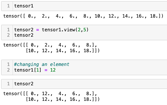
Viewing: PyTorch has [tensor].view, which returns a tensor of different shape while sharing the same data. Suppose tensor1 has shape (3,4) and tensor2=tensor1.view(different compatible shape than tensor1's); in this case, if we change the data in tensor1, tensor2‘s data will also be changed. This happens because tensor2 shares the same memory as tensor1.
Stacking: This stacks tensors on top of each other. torch.stack takes a list of tensors, and a dimension across which the stacking is to be done needs to be provided. The default dimension is dim=0. Here’s an example:

Squeezing and unsqueezing tensors: Squeezing removes dimensions from a tensor with size 1. Below, the first case does not provide any dimension, hence both the 1s are removed; while in the second case, we provide dim=4, which removes only the 1 at the 4th index.

Similarly, unsqueeze adds dimension with size 1 to a tensor. In the example below, we provide dim=1 to torch.unsqueeze to add a new dimension with size 1 at the 1st index.

Permuting: This returns a different view of a tensor with the dimensions permuted. We use torch.permute to get the desired ordering of the dimensions. Here is an example:

That concludes our exploration of the fundamentals of PyTorch and tensors. We’ve discussed some of the most common tensor operations in this post. I recommend bookmarking this documentation page: https://pytorch.org/docs/stable/tensors.html. Make it your go-to resource whenever you encounter concerns while working with PyTorch.
Thanks for making it to the end, and I’ll see you at the next one. Good day!
“If we bring in a scalar and perform multiplication and division,” does this means the broadcasting u spoke on ur past article.
Operation-wise, yes it is broadcasting.
Great article, thank you very much Rabindra.